


Welcome to the fifth part of our Pandas series! In this exciting chapter, we dive headfirst into the world of data aggregation and pivot tables. These powerful techniques are your secret weapons for transforming raw data into valuable insights, making informed decisions, and presenting data in ways that bring clarity to your analysis.
In this blog, we won’t just skim the surface; we’ll actively explore the depths of data manipulation. By the end of this journey, you’ll have the skills to master data grouping, wield aggregation functions like a pro, and craft pivot tables that reshape your data into dynamic, informative summaries. So, let’s roll up our sleeves and dive into the world of Pandas, where data mastery awaits!
Data aggregation is the art of simplifying complex datasets by summarizing and restructuring them, providing essential insights for decision-making. In the world of data analysis, this skill is invaluable. But what’s even more powerful is the ability to reshape data effortlessly, presenting it in ways that make patterns and trends jump off the page. This is where pivot tables come into play.
In this section, we embark on a journey to understand the importance of data aggregation and the pivotal role that pivot tables play in data analysis. We’ll explore how these techniques enable us to distill information, uncover hidden trends, and make data-driven decisions with confidence. So, fasten your seatbelt as we delve into the world of data mastery with Pandas!
Data aggregation and pivot tables are the unsung heroes of data analysis, revolutionizing how we decipher complex datasets. They hold the key to transforming raw data into actionable insights, making informed decisions, and presenting findings with clarity. In this section, we’ll actively delve into why these techniques are pivotal in the realm of data analysis.
Data aggregation isn’t just about simplifying data; it’s about distilling meaning. When working with extensive datasets, aggregation allows us to:
Summarize Information: Aggregation condenses large datasets into meaningful summaries, saving time and reducing complexity.
Spot Trends: By aggregating data, we uncover trends, patterns, and outliers that might be hidden in the noise of raw data.
Make Informed Decisions: Aggregated data serves as a foundation for informed decision-making, providing a clear picture of what’s happening.
Pivot tables are like data sculptors, reshaping information to fit your needs. They actively enable us to:
Reorganize Data: Pivot tables allow for dynamic rearrangement of data, presenting it in a format that emphasizes specific aspects.
Summarize Effectively: They summarize data with ease, providing insights at a glance through customizable calculations and aggregations.
Visualize Relationships: Pivot tables reveal relationships between variables, making it easier to draw conclusions.
Now, let’s actively dive into practical examples and hands-on applications, where the power of data aggregation and pivot tables comes to life.
In the realm of data analysis, the ability to distill vast amounts of information into concise summaries and reshape it for deeper insights is a game-changer. In this section, we actively illuminate the profound significance of summarizing and reshaping data for making insightful decisions.
Summarization acts as a data spotlight, revealing the essential aspects while removing unnecessary complexity:
Efficiency: Summarized data is easier to comprehend and work with, saving time in the analysis process.
Identifying Patterns: By focusing on summaries, we can swiftly spot patterns, trends, and anomalies that might otherwise go unnoticed.
Communication: Summarized data enhances communication by distilling complex information into easily digestible insights, fostering better collaboration among stakeholders.
Consider a scenario where you have a large dataset of daily sales transactions for a retail business. Each row in the dataset represents a single sale, including the date of the sale and the amount of the sale. You want to gain insights into the sales trends over months to inform your inventory management and marketing strategies.
Here’s the code to summarize this sales data by calculating the total sales for each month:

groupby() method to group the sales data based on the month. We extract the month information from the ‘Date’ column using sales_data['Date'].dt.month.sum() function to calculate the sum of sales for each month.Reshaping data allows us to view it from different angles, uncovering relationships and nuances:
Flexibility: Reshaped data adapts to your analytical needs, enabling the exploration of various dimensions.
Comparisons: Different data shapes make it easier to compare variables, uncover correlations, and draw meaningful conclusions.
Customization: Reshaped data is highly customizable, allowing you to create tailor-made reports and visuals.
Imagine you’re conducting a survey with multiple respondents, each providing responses to a set of questions. The survey data is structured with each row representing a respondent’s answer to a specific question, including the respondent’s ID, the question, and their response. You want to analyze this data to gain insights into respondents’ preferences across different questions.
Here’s the code to reshape this survey data into a pivot table format:

pd.pivot_table() function is used to reshape the survey_data DataFrame.aggfunc='first' argument ensures that when there are multiple responses to the same question by the same respondent, we take the ‘first’ response.This revised example demonstrates the use of Pandas to reshape survey data into a pivot table format, allowing for more straightforward analysis and insights extraction.
In the realm of data analysis, one of the most powerful tools at your disposal is the ability to group data based on specific criteria. This process, known as data grouping, enables you to organize and segment your dataset in ways that reveal hidden patterns and insights. In this section, we dive into the world of data grouping with Pandas.
By actively grouping data, you can efficiently analyze subsets, calculate aggregate statistics, and draw meaningful conclusions. Whether you’re exploring sales trends, survey responses, or any other dataset, mastering data grouping with Pandas is a key step towards unraveling the stories hidden within your data. So, let’s embark on this journey of data exploration and discovery together!
In our journey of data exploration with Pandas, once data is neatly grouped, the next step is to actively analyze it. Pandas provides a range of common aggregation functions like sum, mean, and count, which allow us to extract valuable insights from our grouped data. In this section, we will actively explore and apply these aggregation functions to our grouped data, shedding light on their practical utility.
Before we dive into examples, let’s actively introduce some of the most commonly used aggregation functions:
sum(): Computes the sum of values within each group.
mean(): Calculates the mean (average) value within each group.
count(): Counts the number of observations (rows) within each group.
min() and max(): Finds the minimum and maximum values within each group, respectively.
In this illustrative example, we’ll use Pandas, a versatile data manipulation library, to analyze sales data. By grouping transactions based on regions and applying aggregation functions, we can gain valuable insights into sales performance and activity levels across different regions.
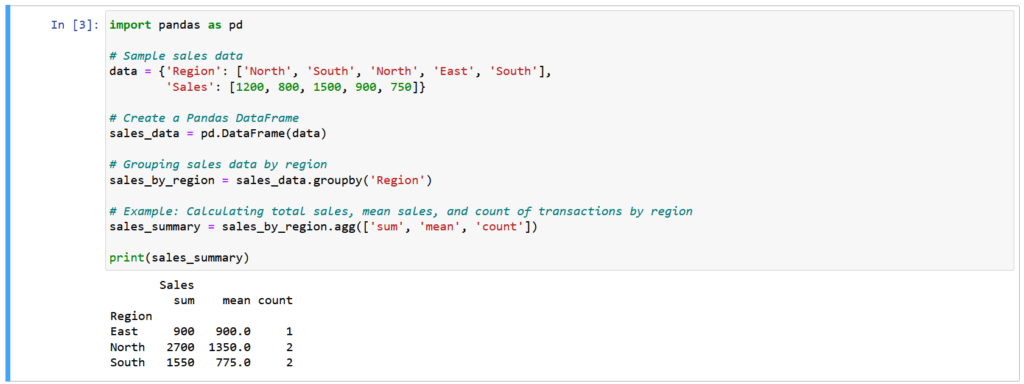
We begin by importing the Pandas library, which is essential for data manipulation and aggregation in this example.
We define a dictionary data containing sales information, including the region and corresponding sales amounts. This dictionary serves as our sample data.
Using the Pandas library, we create a DataFrame called sales_data from the sample data dictionary. This DataFrame organizes the data in a tabular format, making it suitable for analysis.
We use the groupby() method from Pandas to group the sales data by the ‘Region’ column. This step categorizes the data into separate groups based on regions.
sum, mean, and count) to the grouped data (sales_by_region). These functions calculate the following metrics for each region:sum: Computes the total sales amount within each region, indicating which region generates the highest revenue.mean: Calculates the average sales amount per transaction within each region, offering insights into the typical transaction size.count: Counts the number of transactions within each region, revealing the level of sales activity in each area.sales_summary DataFrame to see the aggregated results for each region, which provides insights into the sales performance and activity across different regions.This example demonstrates how Pandas enables us to efficiently group and analyze data, making it a powerful tool for data manipulation and decision-making.
The application of aggregation functions goes beyond just summing and averaging numbers. It actively helps us draw practical conclusions from our data. Whether you’re analyzing sales figures, survey responses, or any dataset, mastering these aggregation functions empowers you to extract meaningful insights actively.
So, let’s roll up our sleeves and embark on an active exploration of aggregation functions with Pandas, unraveling valuable insights within our grouped data.
In this section, we embark on an active exploration of the GroupBy method’s capabilities in Pandas. By actively applying aggregate functions and discussing advanced aggregation techniques, we’ll unlock the potential of data aggregation for insightful analysis. Additionally, we’ll illustrate the use of the agg() method, a versatile tool for performing multiple aggregations in a single step.
Custom aggregation functions are a fundamental component of Pandas, a versatile data manipulation library in Python. They offer a remarkable degree of flexibility, allowing you to define your own logic for summarizing data. This flexibility is invaluable because it enables you to address nuanced data analysis challenges that often arise in real-world scenarios.
Python Functions for Custom Aggregation:
Python functions provide a robust and flexible approach to creating custom aggregation functions in Pandas. In this example, we’ll create a custom aggregation function using a Python function to calculate the weighted average of product ratings in a sales dataset.
Let’s assume we have a sales dataset that includes product ratings (on a scale of 1 to 5) and the number of units sold for each product. We want to calculate the weighted average rating, where products with higher sales count have a more significant impact on the average rating.
Here’s how you can do it:
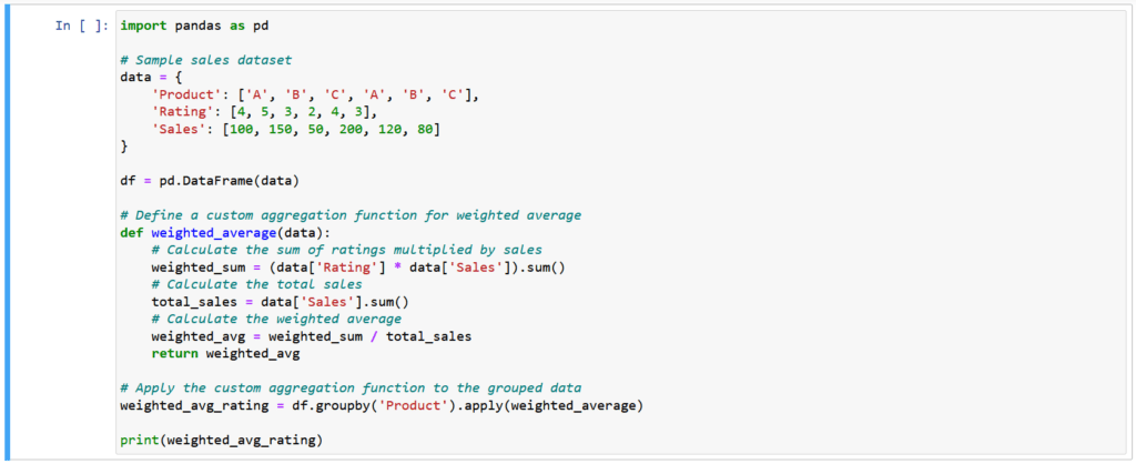

We create a sample sales dataset using a dictionary.
Then we define a custom aggregation function named weighted_average that calculates the weighted average of product ratings. It does this by summing the products of ratings and sales for each product and dividing by the total sales.
Using groupby(), we group the data by the ‘Product’ column.
We apply the weighted_average function to each group, resulting in the weighted average rating for each product.
Finally, we print the weighted average ratings for each product.
This example showcases how Python functions can be used to create custom aggregation functions for specific data summarization needs. The flexibility of Python functions allows you to implement complex summarization logic tailored to your dataset.
Lambda expressions provide a concise and on-the-fly approach to creating custom aggregation functions in Pandas. In this example, we’ll use a lambda expression to calculate the total profit for each product in a sales dataset.
Suppose we have a sales dataset containing product names, prices, and the number of units sold. We want to calculate the total profit for each product, where profit is calculated as the product of price and quantity sold.
Here’s how you can achieve this using a lambda expression:
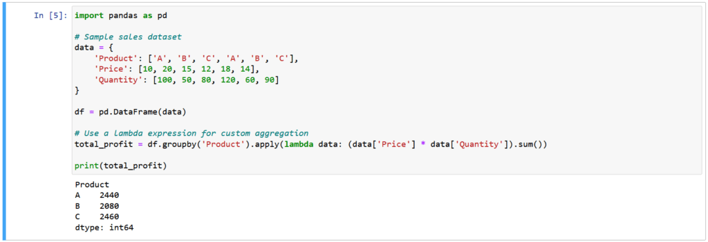
We create a sample sales dataset using a dictionary, including product names, prices, and quantities sold.
Then we use a lambda expression within the groupby() function to define a custom aggregation function. The lambda expression calculates the total profit for each product by multiplying the price and quantity sold and then summing these values.
The groupby('Product') groups the data by the ‘Product’ column.
We apply the lambda expression to each group, resulting in the total profit calculation for each product.
Finally, we print the total profit for each product.
This example demonstrates how lambda expressions are a concise choice for creating custom aggregation functions, especially for one-time-use scenarios. They allow you to define custom logic on the spot, providing flexibility and efficiency in your data analysis workflow.
In this example, we’ll demonstrate how to calculate a custom median for sales data grouped by region. While Pandas provides various built-in aggregation functions, computing the median is not one of them. Therefore, we’ll create a custom aggregation function to find the median sales value for each region.
Suppose we have a sales dataset with information about sales figures and the corresponding regions. Our goal is to determine the median sales value for each region.
Here’s how you can achieve this using a custom aggregation function:
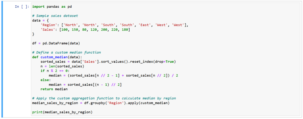
Output:

We create a sample sales dataset with ‘Region’ and ‘Sales’ columns.
Then we define a custom aggregation function named custom_median. This function calculates the median of sales values for each region. It sorts the sales values, handles even and odd numbers of data points, and returns the median.
groupby('Region') to group the data by region.
We apply the custom_median function to each group, resulting in the median sales calculation for each region.
Finally, we print the median sales values for each region.
This example showcases how to create and apply a custom aggregation function to compute the median, providing valuable insights for your data analysis needs.
In this example, we’ll use a lambda expression-based custom aggregation function to calculate the sales range within each region of a sales dataset.
Example: Calculating Custom Sales Range
Imagine we have a sales dataset containing information about sales figures and the corresponding regions. Our goal is to determine the sales range (the difference between the maximum and minimum sales) for each region.
Here’s how you can achieve this using a custom aggregation function with a lambda expression:
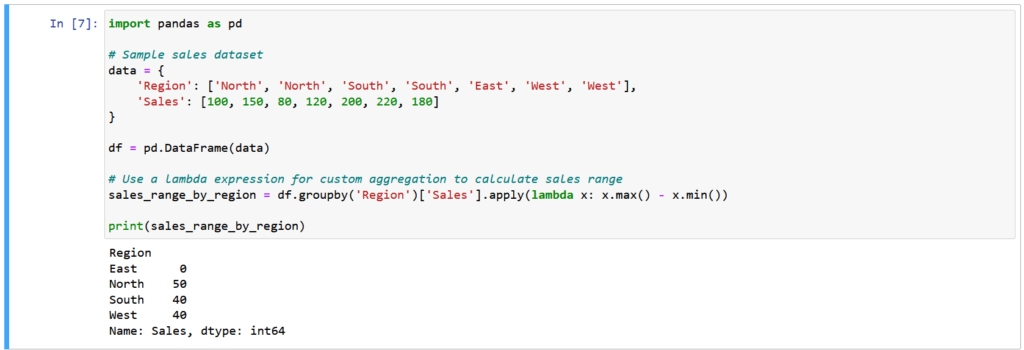
We create a sample sales dataset with ‘Region’ and ‘Sales’ columns.
Lambda expression-based custom aggregation function within groupby('Region') to calculate the sales range for each region. The lambda expression calculates the difference between the maximum and minimum sales within each group.
The result is a Series that displays the sales range for each region.
We print the sales range for each region.
This example demonstrates how to efficiently use a lambda expression for a custom aggregation function to calculate the sales range within different regions of your dataset, providing valuable insights into your data analysis.
Custom aggregation functions are not just theoretical concepts; they play a pivotal role in real-world data analysis. Whether you’re analyzing sales data, customer behavior, or any other domain, the ability to tailor your summarization techniques ensures that you extract the precise insights needed for informed decision-making.
By mastering custom aggregation functions, you empower yourself to conquer the complexities of data analysis, unlocking a world of possibilities for extracting valuable insights from your datasets.
agg() MethodIn this section, we actively delve into the agg() method in Pandas, a powerful tool that streamlines data analysis by enabling you to perform multiple aggregations in a single step. This method proves invaluable when you seek comprehensive insights from your data without the need for repetitive or convoluted code.
agg() MethodThe agg() method, short for “aggregate,” is a versatile function in Pandas that empowers you to apply multiple aggregation functions to your data simultaneously. It simplifies and accelerates the process of summarizing and gaining insights from datasets, making it an indispensable tool for efficient data analysis.
One of the standout features of the agg() method is its ability to perform multiple aggregations on one or more columns within your DataFrame. This capability drastically reduces the need for writing redundant code, streamlining your data analysis workflow.
Comprehensive Sales Summary by Region:
In this example, we’ll demonstrate the power of the agg() method by obtaining a comprehensive sales summary for different regions in a sales dataset. We want to efficiently calculate the sum, mean, maximum, and minimum sales figures in a single operation.
Suppose we have a sales dataset with ‘Region’ and ‘Sales’ columns. Our objective is to generate a summary that includes the total sales, average sales, maximum sales, and minimum sales for each region using the agg() method.
Here’s how you can achieve this:
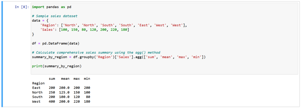
We create a sample sales dataset with ‘Region’ and ‘Sales’ columns.
We use the groupby('Region') method to group the data by region.
With the agg() method, we specify a list of aggregation functions (‘sum’, ‘mean’, ‘max’, ‘min’) to calculate multiple summary statistics for each region simultaneously.
The result is a DataFrame that displays the total sales, average sales, maximum sales, and minimum sales for each region.
We print the comprehensive sales summary by region.
This example showcases the efficiency and versatility of the agg() method in calculating multiple aggregation functions in a single step, providing valuable insights into sales performance by region.
The agg() method is not merely a convenience but a practical necessity in data analysis. It empowers data analysts to efficiently extract meaningful insights from diverse datasets without the need for convoluted code or repetitive calculations. This efficiency is particularly crucial when dealing with extensive data, where time and accuracy are of the essence.
By mastering the agg() method, you gain a valuable tool that enhances your data analysis capabilities, allowing you to extract a wealth of information from your datasets in a single, elegant operation.
In this section, we will explore the concept of pivot tables, a powerful tool for data summarization in Pandas. Pivot tables allow us to reshape and summarize data for improved readability and analysis. We’ll learn how to create pivot tables using the pivot_table() method and illustrate their utility through real-world examples in data reporting.
Let’s dive into the world of pivot tables and discover how they can enhance our data analysis and presentation.
Pivot tables are a remarkable feature in Pandas that empower data analysts to efficiently summarize and gain insights from complex datasets. These versatile tables enable us to aggregate, reorganize, and simplify large amounts of data, making it easier to comprehend and analyze.
At their core, pivot tables allow us to:
Aggregate Data: Pivot tables provide a structured way to perform aggregation operations such as sum, mean, count, and more on selected columns, making it simple to calculate key statistics.
Restructure Data: They enable us to reshape data by rearranging rows and columns, providing a clearer view of specific aspects of the dataset.
Enhance Readability: Pivot tables enhance the presentation of data, making it more readable and facilitating data-driven decision-making.
In the upcoming sections, we will delve deeper into creating pivot tables, actively reshaping data, and providing real-world examples that highlight their indispensable role in data reporting and analysis.
pivot_table() MethodPandas provides the pivot_table() method, which is a versatile tool for generating pivot tables from your dataset. This method enables you to create customized pivot tables by specifying the columns for rows, columns, values, and aggregation functions. Here’s a breakdown of the process:
Data Selection: Begin by selecting the dataset (DataFrame) that you want to create a pivot table from. Ensure that your DataFrame contains the relevant columns for the pivot table’s rows, columns, and values.
Specify Rows and Columns: Use the index and columns parameters of the pivot_table() method to determine which columns should serve as rows and columns in the pivot table. This defines the structure of your table.
Choose Values to Aggregate: Indicate the column(s) that contain the data you want to summarize. These values will be aggregated based on the row and column combinations.
Select Aggregation Functions: Specify the aggregation function(s) to apply to the selected values. Common aggregation functions include ‘sum’, ‘mean’, ‘count’, ‘max’, ‘min’, and more. You can use multiple aggregation functions if needed.
Create the Pivot Table: Execute the pivot_table() method with the specified parameters to generate your customized pivot table.
Review and Analyze: Once you have your pivot table, you can review the summarized data and use it for in-depth analysis, reporting, and decision-making.
By understanding how to effectively use the pivot_table() method, you can transform your dataset into a structured and insightful pivot table that provides valuable insights and facilitates data exploration.
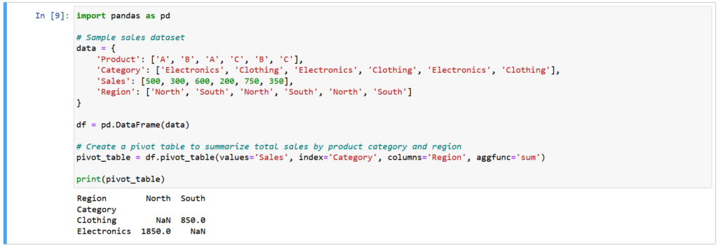
We start with a sample sales dataset that includes columns for ‘Product’, ‘Category’, ‘Sales’, and ‘Region’.
Using the pivot_table() method, we specify the following parameters:
values='Sales': We want to summarize the ‘Sales’ column.index='Category': We set the ‘Category’ column as the rows of the pivot table.columns='Region': The ‘Region’ column becomes the columns of the pivot table.aggfunc='sum': We choose to calculate the sum of sales for each combination of product category and region.The result is a pivot table that displays the total sales for each product category (‘Clothing’ and ‘Electronics’) in different regions (‘North’ and ‘South’). This structured table simplifies the analysis of sales data by providing a clear overview of sales performance across categories and regions.
By utilizing the pivot_table() method in Pandas, you can efficiently generate customized pivot tables tailored to your data analysis needs.
In this fifth part of our Python series, we’ve delved deep into the art of grouping and aggregating data using Pandas. Let’s summarize the key takeaways from this journey:
groupby():We began by introducing the versatile groupby() function, a pivotal tool in Pandas for grouping data based on specific criteria. This function forms the foundation for aggregating and analyzing data efficiently.
We explored essential aggregation functions such as sum, mean, and count, which empower us to gain insights by summarizing grouped data. These functions play a crucial role in extracting meaningful information from complex datasets.
We unlocked the potential of custom aggregation functions, providing the flexibility to tailor data summarization to our unique needs. Python functions and lambda expressions emerged as valuable tools for crafting custom aggregation logic.
We ventured into the world of pivot tables and cross-tabulations, demonstrating how they can reshape and enhance the readability of data. These techniques are indispensable for generating clear and insightful summaries.
As we move forward in our Python series, anticipate more advanced data manipulation techniques, real-world applications, and opportunities to sharpen your data analysis skills. Stay tuned for the next chapter as we continue our exploration of Python’s data-handling capabilities.


We provide online certification in Data Science and AI, Digital Marketing, Data Analytics with a job guarantee program. For more information, contact us today!
Courses
1stepGrow
Anaconda | Jupyter Notebook | Git & GitHub (Version Control Systems) | Python Programming Language | R Programming Langauage | Linear Algebra & Statistics | ANOVA | Hypothesis Testing | Machine Learning | Data Cleaning | Data Wrangling | Feature Engineering | Exploratory Data Analytics (EDA) | ML Algorithms | Linear Regression | Logistic Regression | Decision Tree | Random Forest | Bagging & Boosting | PCA | SVM | Time Series Analysis | Natural Language Processing (NLP) | NLTK | Deep Learning | Neural Networks | Computer Vision | Reinforcement Learning | ANN | CNN | RNN | LSTM | Facebook Prophet | SQL | MongoDB | Advance Excel for Data Science | BI Tools | Tableau | Power BI | Big Data | Hadoop | Apache Spark | Azure Datalake | Cloud Deployment | AWS | GCP | AGILE & SCRUM | Data Science Capstone Projects | ML Capstone Projects | AI Capstone Projects | Domain Training | Business Analytics
WordPress | Elementor | On-Page SEO | Off-Page SEO | Technical SEO | Content SEO | SEM | PPC | Social Media Marketing | Email Marketing | Inbound Marketing | Web Analytics | Facebook Marketing | Mobile App Marketing | Content Marketing | YouTube Marketing | Google My Business (GMB) | CRM | Affiliate Marketing | Influencer Marketing | WordPress Website Development | AI in Digital Marketing | Portfolio Creation for Digital Marketing profile | Digital Marketing Capstone Projects
Jupyter Notebook | Git & GitHub | Python | Linear Algebra & Statistics | ANOVA | Hypothesis Testing | Machine Learning | Data Cleaning | Data Wrangling | Feature Engineering | Exploratory Data Analytics (EDA) | ML Algorithms | Linear Regression | Logistic Regression | Decision Tree | Random Forest | Bagging & Boosting | PCA | SVM | Time Series Analysis | Natural Language Processing (NLP) | NLTK | SQL | MongoDB | Advance Excel for Data Science | Alteryx | BI Tools | Tableau | Power BI | Big Data | Hadoop | Apache Spark | Azure Datalake | Cloud Deployment | AWS | GCP | AGILE & SCRUM | Data Analytics Capstone Projects
Anjanapura | Arekere | Basavanagudi | Basaveshwara Nagar | Begur | Bellandur | Bommanahalli | Bommasandra | BTM Layout | CV Raman Nagar | Electronic City | Girinagar | Gottigere | Hebbal | Hoodi | HSR Layout | Hulimavu | Indira Nagar | Jalahalli | Jayanagar | J. P. Nagar | Kamakshipalya | Kalyan Nagar | Kammanahalli | Kengeri | Koramangala | Kothnur | Krishnarajapuram | Kumaraswamy Layout | Lingarajapuram | Mahadevapura | Mahalakshmi Layout | Malleshwaram | Marathahalli | Mathikere | Nagarbhavi | Nandini Layout | Nayandahalli | Padmanabhanagar | Peenya | Pete Area | Rajaji Nagar | Rajarajeshwari Nagar | Ramamurthy Nagar | R. T. Nagar | Sadashivanagar | Seshadripuram | Shivajinagar | Ulsoor | Uttarahalli | Varthur | Vasanth Nagar | Vidyaranyapura | Vijayanagar | White Field | Yelahanka | Yeshwanthpur
Mumbai | Pune | Nagpur | Delhi | Gurugram | Chennai | Hyderabad | Coimbatore | Bhubaneswar | Kolkata | Indore | Jaipur and More