Exploring NumPy in Python: Broadcasting

Table of Contents

Introduction:

Welcome back to the fourth part of our comprehensive NumPy series! If you’ve been following along, you’ve already gained a solid understanding of the basics, essential techniques, and data manipulation capabilities that NumPy offers.

In this part of our journey through NumPy, we’re diving into the deep end. Here, we’ll actively explore advanced concepts and harness the remarkable power of major NumPy broadcasting. These are the backbone of complex operations, data analysis, and scientific computations. Whether you identify as a data scientist, engineer, or Python enthusiast, rest assured that these advanced NumPy skills will elevate your proficiency to new heights.

Broadcasting: Simplifying Array Operations in NumPy

NumPy, “broadcasting” is the secret sauce that allows you to perform element-wise operations on arrays with different shapes, making your life as a data scientist or Python developer considerably easier. In this section, we’ll demystify broadcasting and show you how it can simplify array operations.

How Broadcasting Works


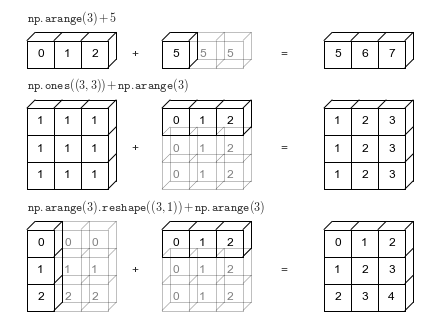
Picture two arrays: one with shape (3, 3) and another with shape (1, 3), and you want to add them. Traditionally, they’d need the same shape. But broadcasting lets NumPy handle this with ease.

Broadcasting Rules


NumPy abides by a set of rules for broadcasting. It kicks off by comparing input array dimensions. When they don’t match, NumPy adds a “virtual” dimension of size 1 to the smaller array, harmonizing their compatibility.

00
Broadcasting Rules in NumPy


Rule 1: Dimension Comparison

  • NumPy compares the dimensions of input arrays.
  • It starts with the trailing dimensions and works backward.
  • In case dimensions match or are size-1 (meaning one of them has size 1), broadcasting is possible.


Rule 2: Dimension Expansion

  • If dimensions don’t match, NumPy adds “virtual” dimensions of size 1 to the smaller array.
  • This expansion ensures both arrays have the same number of dimensions.


Rule 3: Size Compatibility

  • Broadcasting continues if either array’s dimensions match or one of them has a size of 1.
  • If neither condition is met, broadcasting raises an error.


Rule 4: Shape Compatibility

  • After dimension expansion, arrays’ shapes must align element-wise.
  • If they don’t, broadcasting raises an error.


These systematic rules guide broadcasting in NumPy, making it easier to grasp and apply in your array operations.

Harnessing Broadcasting’s Might


Broadcasting simplifies operations like addition, subtraction, multiplication, and division, and extends its prowess to advanced tasks like reshaping and slicing. It shines in handling vast datasets and operations on data subsets.

Seamless Integration with Major NumPy Functions

Broadcasting doesn’t stand alone. It seamlessly integrates with major NumPy functions like np.sum, np.mean, and np.max, making complex computations remarkably manageable.


In the upcoming examples, we’ll unveil broadcasting’s versatility in various scenarios and demonstrate its practical synergy with major NumPy functions. Get ready to unlock broadcasting’s potential and streamline your array operations!

Broadcasting in Action: Examples and Applications

Now, let’s put broadcasting into practice with examples that illustrate its versatility and real-world applications.

Example 1: Broadcasting for Element-Wise Operations

Consider a scenario where we have a 2D array A representing temperature data for different days of the week with the shape (3, 3), and a 1D array B containing temperature adjustments for each day with the shape (3,). If we want to calculate the adjusted temperatures for each day by adding the adjustments from B, broadcasting simplifies the task.

01

In this example, broadcasting automatically expands the dimensions of B to match the shape of A, enabling us to perform element-wise addition seamlessly.

Explanation:
  • Broadcasting starts by comparing the dimensions of the input arrays, Aand B. They differ in shape, with A having a shape of (3, 3) and B having a shape of (3,). To make them compatible, broadcasting adds a “virtual” dimension of size 1 to B, changing its shape to (1, 3).


  • Now that the dimensions are compatible, NumPy performs element-wise addition between Aand the broadcasted B. It adds each element of B to the corresponding row in A, resulting in the adjusted_temperatures


  • The resulting array adjusted_temperaturescontains the adjusted temperatures for each day, where the adjustments from B have been applied element-wise.

This demonstrates how broadcasting simplifies element-wise operations, even when the shapes of the input arrays differ, making it a powerful tool for data manipulation in NumPy.

Example 2: Broadcasting in Aggregation

Consider a scenario where we have a 2D array scores representing student scores in different subjects with the shape (3, 4). We want to calculate the mean score for each student, which involves adding up the scores along the columns. Broadcasting simplifies this aggregation task.

02

In this example, broadcasting allows us to add up the scores along the columns effortlessly to calculate the mean score for each student.

Explanation:
  • We start with a 2D array scores representing student scores, where each row corresponds to a student, and each column represents a subject.

  • To calculate the mean score for each student, we use the np.mean function along axis=1. This indicates that we want to perform the mean operation along the columns (i.e., for each student).

  • Broadcasting comes into play when we apply np.mean to the scores array. It effectively treats each row as a separate entity and aggregates the scores along the columns, resulting in an array mean_scores containing the mean score for each student.

  • It simplifies the aggregation process, making it concise and easy to understand. It’s a powerful feature when dealing with multi-dimensional arrays and aggregation operations in NumPy.

Example 3: Broadcasting for Normalization

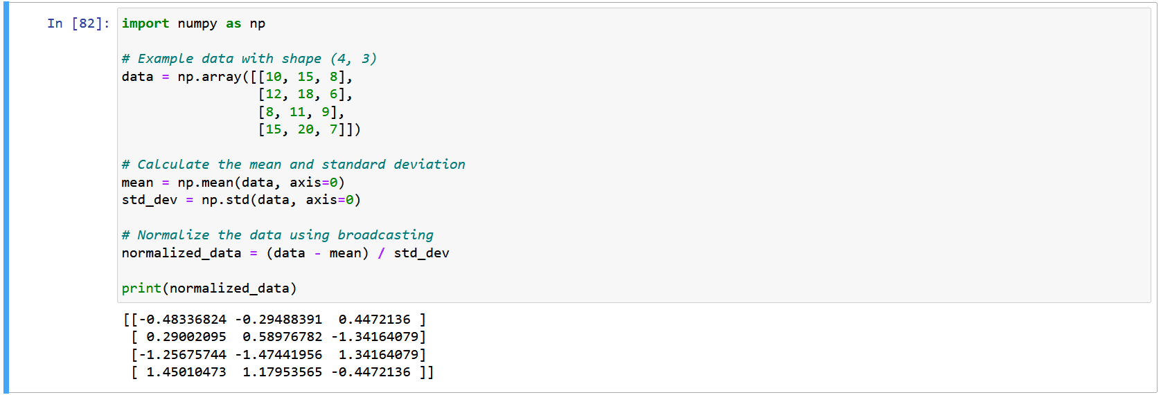
Data preprocessing frequently involves normalizing data to have a mean of zero and a standard deviation of one. Broadcasting in NumPy simplifies this task.

03

In this example, broadcasting allows us to efficiently normalize the data by subtracting the mean and dividing by the standard deviation for each column.

Explanation:

  • We begin with an example dataset data, which has a shape of (4, 3), representing four samples with three features each.

  • To normalize the data, we calculate the mean and standard deviation along axis=0 using the np.mean and np.std functions. This computes the mean and standard deviation for each feature (column).

  • Broadcasting plays a crucial role when we normalize the data. The expression (data - mean) / std_dev is applied element-wise, meaning that for each element in data, it subtracts the corresponding mean and then divides by the corresponding standard deviation.

  • It ensures that the subtraction and division operations are carried out consistently across all elements, resulting in a normalized dataset normalized_data with a mean of zero and a standard deviation of one for each feature.

  • The use of broadcasting also simplifies the normalization process, making the code concise and comprehensible. It’s a powerful tool for performing element-wise operations on arrays with different shapes.

Combining Broadcasting with NumPy Functions

To harness the full potential of broadcasting, let’s explore how it seamlessly integrates with some major NumPy functions.

Example 4: Broadcasting with np.sum

Imagine a scenario where you’re dealing with a 2D array ‘data’ that records daily sales for various products. This ‘data’ array has a shape of (5, 7), signifying five products and seven days of sales data.

Objective: Calculate the total sales for each product during the seven days.

Example:

04
Explanation:
  • We import NumPy as ‘np’ to utilize its functions.
  • The ‘data’ array simulates the sales figures for five different products over seven days.
  • By applying the ‘np.sum’ function with ‘axis=1’, we perform a summation operation along the columns (days) of the ‘data’ array.
  • This results in a concise ‘total_sales’ array that reveals the total sales for each product over the specified time frame.

Broadcasting, as demonstrated here, simplifies complex tasks, making NumPy an invaluable tool for data processing and analysis.

Example 5: Broadcasting with np.max

Let’s envision a scenario where you have a 1D array ‘temperatures’ that stores the daily temperatures recorded over a month. The array ‘temperatures’ holds 30 elements, each representing the temperature on a specific day.

Objective: Determine the hottest temperature recorded during this month.

Example:

05
Explanation:
  • We first import NumPy as ‘np’ to access its functions.
  • The ‘temperatures’ array holds daily temperature data for a month, featuring 30 elements.
  • By employing the ‘np.max’ function, we conduct a broadcasting operation to identify the highest temperature recorded during this period.
  • The result, ‘hottest_temperature’, succinctly reveals the hottest temperature, simplifying the process of finding extreme values within an array.

This example underscores the versatility of broadcasting in conjunction with major NumPy functions, enhancing the efficiency of tasks involving element-wise operations.

Example 6: Broadcasting with np.mean

Consider a scenario where you possess a 2D array ‘scores’ that records test scores for students across various subjects. You aim to assess the students’ overall performance by determining the mean score for each individual.

Example:

06
Explanation:
  • We initiate the example by importing NumPy as ‘np’ to leverage its functionality.
  • The ‘scores’ array encapsulates test scores for students, presented in a 2D format with students in rows and subjects in columns.
  • Employing the ‘np.mean’ function, we apply broadcasting to ascertain the mean score for each student. The ‘axis=1’ argument ensures we calculate the mean across subjects for each student.
  • The outcome, ‘mean_scores,’ provides a concise representation of the students’ overall performance. This demonstrates broadcasting’s role in streamlining complex tasks like aggregating data across different dimensions, thereby enhancing data analysis efficiency.

This example underscores how broadcasting seamlessly integrates with major NumPy functions, facilitating intricate operations involving element-wise computations.

Example 7: Broadcasting with np.multiply

Consider a scenario where you possess a 2D array ‘prices,’ which records the prices of different items in a store, and a 1D array ‘quantities,’ representing the quantity of each item sold. The objective is to compute the total revenue generated for each item.

Example:

07
Explanation:
  • This example commences by importing NumPy as ‘np’ to make use of its array operations.
  • The ‘prices’ array captures the pricing information of various store items, forming a 1D array.
  • Correspondingly, the ‘quantities’ array holds data regarding the quantity of each item sold, structured as a 1D array.
  • To determine the total revenue generated for each item, we utilize the ‘np.multiply’ function while taking advantage of broadcasting. This operation multiplies the prices by the respective quantities for each item, offering a concise representation of the revenue generated for each item.
  • The result, ‘revenue_per_item,’ showcases the effectiveness of broadcasting in simplifying complex tasks such as performing element-wise operations on arrays with distinct shapes.

Important Points about Broadcasting:


  1. Efficiency: Broadcasting enables efficient element-wise operations without the need to create additional copies of data, which can be crucial when dealing with large datasets.

  2. Memory Conservation: It helps conserve memory by avoiding the creation of redundant arrays, making NumPy operations memory-efficient.

  3. Broadcasting Rules: Understanding the rules of broadcasting is essential for error-free operations. Keep in mind that dimensions should be compatible or equal for broadcasting to work correctly.

  4. Applications: Broadcasting simplifies tasks like reshaping, slicing, and mathematical operations, making it a powerful tool for data manipulation.

  5. Integration with NumPy Functions: It seamlessly integrates with major NumPy functions like np.sum, np.mean, and np.max, enhancing their usability and readability.

  6. Readable Code: Utilizing broadcasting can lead to more concise and readable code, improving the maintainability of your projects.


Mastering broadcasting and combining it with NumPy’s extensive functions equips you to tackle complex data analysis and scientific computing tasks efficiently. This foundational knowledge significantly enhances your proficiency in Python, opening up new possibilities for your projects.

The Bottom Line

In conclusion, broadcasting is a powerful feature of NumPy that simplifies element-wise operations on arrays with different shapes. By understanding the broadcasting rules and integrating it with major NumPy functions, you can efficiently manipulate data, conserve memory, and write more readable code.


Efficient broadcasting is especially valuable when dealing with large datasets and performing complex calculations. Whether you’re normalizing data, aggregating values, or performing mathematical operations, broadcasting streamlines the process. If you enjoyed the blog visit 1stepgrow.